scatter

📝Syntax

scatter(x, y)
scatter(x, y, sz)
scatter(x, y, sz, c)
scatter(..., 'filled')
scatter(..., marker)
scatter(ax, ...)
scatter(..., propertyName, propertyValue)
s = scatter(...)

📥Input Arguments

Parameter	Description
X	x-coordinates: vector or matrix.
Y	y-coordinates: vector or matrix.
sz	Marker size: numeric scalar, vector, [] (default: 36)
c	Marker color: short color name, color name, RGB triplet or vector of colormap indices
ax	a scalar graphics object value: parent container, specified as a axes.
propertyName	a scalar string or row vector character. See scatter properties for the property list.
propertyValue	a value.

📤Output Arguments

Parameter	Description
s	a graphics object: scatter type or array of scatter.

📄Description

scatter(x, y) generates a scatter plot by placing circular markers at the coordinates defined by the vectors x andy.

If you intend to display a single dataset, ensure that both x andy are vectors of the same length.

To visualize multiple datasets on a shared set of axes, you can achieve this by using a matrix for either x ory, while keeping the other as a vector.

This allows you to overlay or compare multiple datasets within the same plot.

See scatter properties for the complete property list.

💡Examples

f = figure();
theta = linspace(0,1,600);
x = exp(theta).*sin(110*theta);
y = exp(theta).*cos(110*theta);
s = scatter(x,y ,'filled');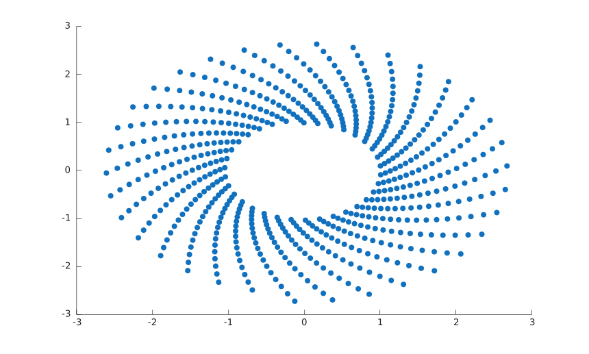

f = figure();
x = linspace(0,3*pi,255);
y = cos(x) + rand(1,255);
sz = 1:255;
c = 1:length(x);
scatter(x, y, sz, c, 'd', 'filled')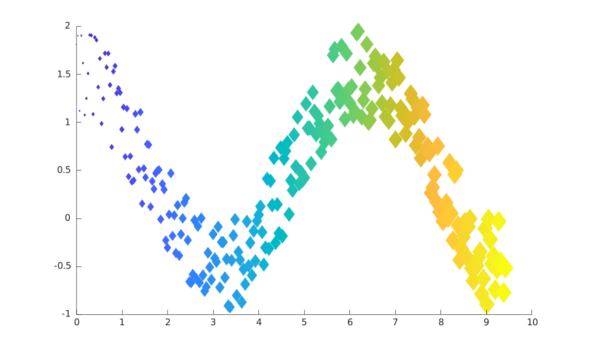

f = figure();
x = linspace(0, 3*pi, 255);
y = cos(x) + rand(1, 255);
c = linspace(1,10,length(x));
scatter(x, y, [], c, 'filled')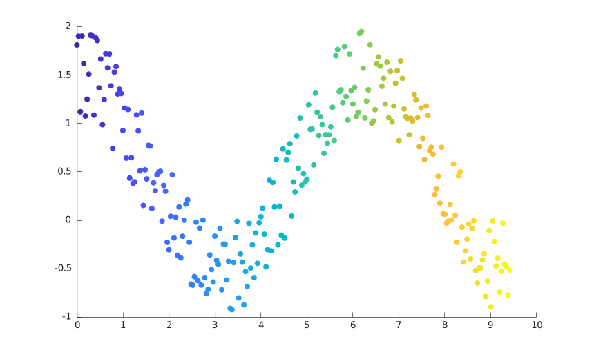

f = figure();
theta = linspace(0,2*pi,244);
x = sin(theta) + 0.75*rand(1,244);
y = cos(theta) + 0.75*rand(1,244);
sz = 45;
scatter(x,y,sz,'MarkerEdgeColor',[0 .6 .5], 'MarkerFaceColor',[0 .6 .7],  'LineWidth',3.5)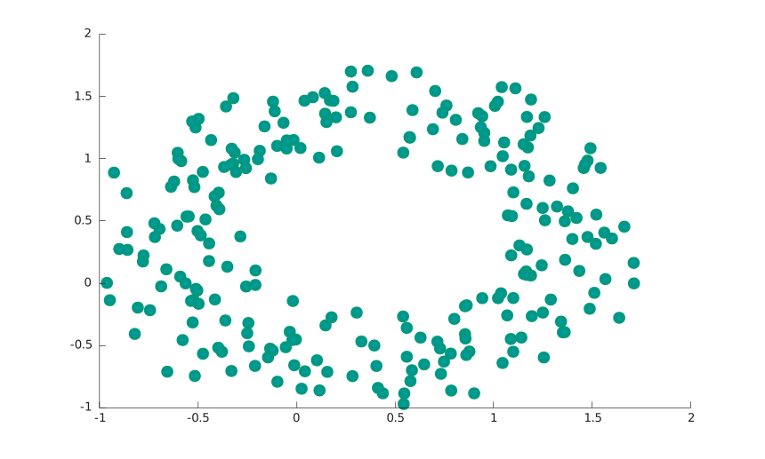

f = figure(),
x = linspace(0,3*pi,200);
y = cos(x) + rand(1,200);
% Top plot
ax1 = subplot(2,1, 1);
scatter(ax1,x,y)
% Bottom plot
ax2 = subplot(2,1, 2);
scatter(ax2,x,y,'filled','d')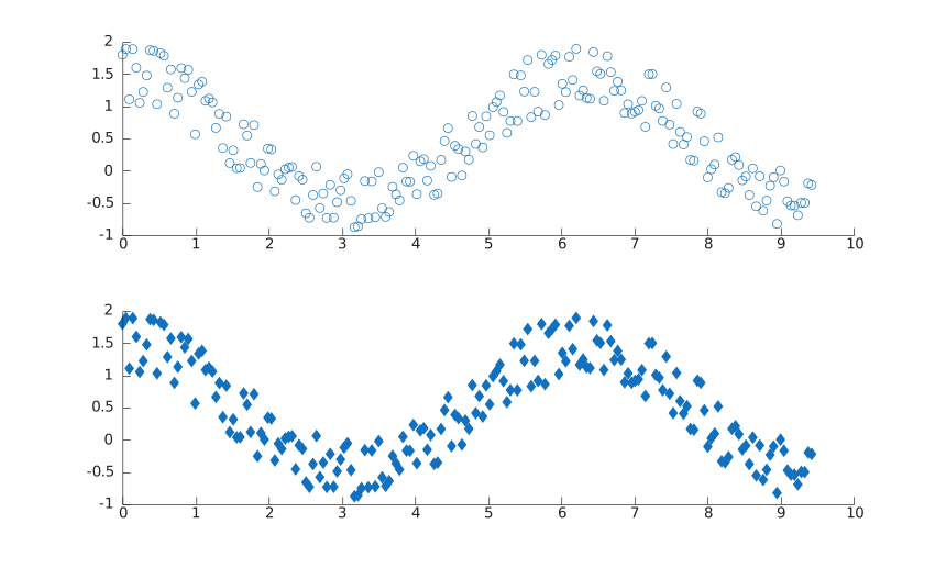

f = figure();
x = rand(500,5);
y = randn(500,5) + (5:5:25);
s = scatter(x,y, 'filled');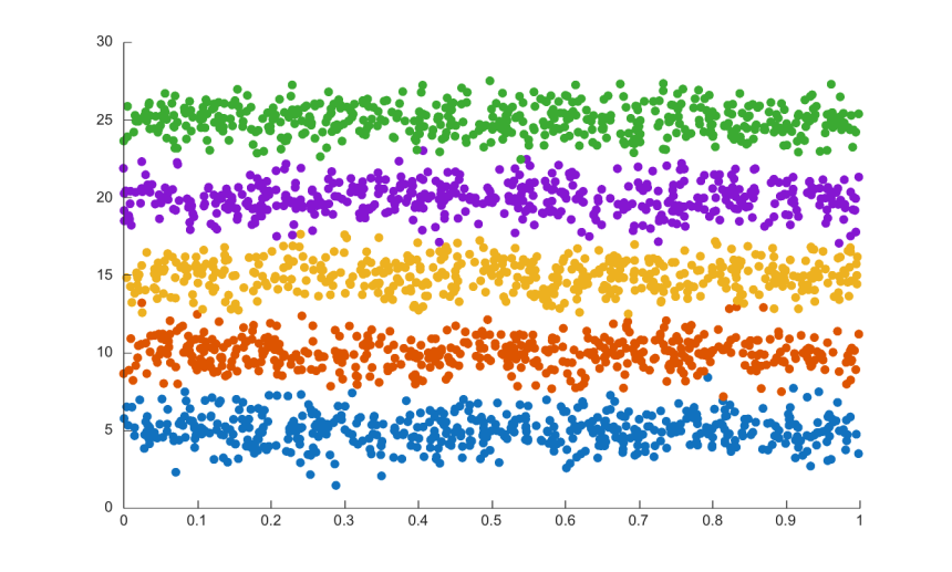

f = figure();
% Create figure
hold on;
% Settings
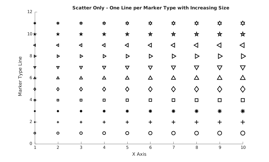
nPoints = 10; % Number of points per marker type
markers = {'o', '+', '*', 's', 'd', '^', 'v', '>', '<', 'p', 'h'};
sizesMin = 20; % Minimum size
sizesMax = 100; % Maximum size
% X positions
x = linspace(1, 10, nPoints);
% Fixed color
fixedColor = [0 0 0]; % black
% Plot each marker type
for m = 1:numel(markers)
    y = m * ones(size(x)); % Constant Y for each marker type
    sizes = linspace(sizesMin, sizesMax, nPoints); % Increasing sizes
    % Scatter points
    scatter(x, y, sizes, ...
        'Marker', markers{m}, ...
        'MarkerEdgeColor', fixedColor, ...
        'MarkerFaceColor', 'none', ...
        'LineWidth', 1.5);
end
title('Scatter Only - One Line per Marker Type with Increasing Size');
xlabel('X Axis');
ylabel('Marker Type Line');
ylim([0 numel(markers)+1]);
hold off;

🕔Version History

Version	Description
1.0.0	initial version
1.12.0	color name and short color name managed.
1.14.0	Scatter is a graphics object with Properties.