Examples
Cluster two dense groups and one noise observation.
X = [0 0; 0 0.1; 5 5; 5 5.1; 10 10];
[idx, corepts] = dbscan(X, 0.2, 2)
Return only the cluster labels.
X = [0 0; 0 0.1; 5 5; 5 5.1];
idx = dbscan(X, 0.2, 2)
Use a larger minpts value to mark all observations as noise.
X = [0; 0.1];
[idx, corepts] = dbscan(X, 1, 3)
Points exactly at epsilon are included in the neighborhood.
X = [0; 1; 2];
idx = dbscan(X, 1, 2)
Cluster duplicate rows with a very small radius.
X = [1 1; 1 1; 1 1; 5 5];
[idx, corepts] = dbscan(X, 1e-12, 3)
Use squared Euclidean distance.
X = [0 0; 0.1 0.05; 5 5; 5.05 5.05];
idx = dbscan(X, 1, 2, 'Distance', 'squaredeuclidean')
Use city block distance.
X = [0 0; 0.1 0.05; 5 5; 5.05 5.05];
idx = dbscan(X, 0.2, 2, 'Distance', 'cityblock')
Use Chebychev distance.
X = [0 0; 0.1 0.05; 5 5; 5.05 5.05];
idx = dbscan(X, 0.1, 2, 'Distance', 'chebychev')
Use Minkowski distance with exponent 1.
X = [0 0; 0.1 0.05; 5 5; 5.05 5.05];
idx = dbscan(X, 0.2, 2, 'Distance', 'minkowski', 'P', 1)
Use standardized Euclidean distance with an explicit scale.
X = [0 0; 0.1 0.05; 5 5; 5.05 5.05];
idx = dbscan(X, 0.2, 2, 'Distance', 'seuclidean', 'Scale', [1 1])
Use Mahalanobis distance with an explicit covariance matrix.
X = [0 0; 0.1 0.05; 5 5; 5.05 5.05];
idx = dbscan(X, 0.2, 2, 'Distance', 'mahalanobis', 'Cov', eye(2))
Use cosine distance to group observations with the same direction.
X = [1 0; 2 0; 0 1; 0 2];
idx = dbscan(X, 0.01, 2, 'Distance', 'cosine')
Use correlation distance.
X = [1 2; 2 3; 10 9; 11 10];
idx = dbscan(X, 0.01, 2, 'Distance', 'correlation')
Use Spearman distance.
X = [1 2; 2 3; 10 9; 11 10];
idx = dbscan(X, 0.01, 2, 'Distance', 'spearman')
Use Hamming distance on binary-valued rows.
X = [1 0 0; 1 0 0; 0 1 0; 0 1 0];
idx = dbscan(X, 0.01, 2, 'Distance', 'hamming')
Use Jaccard distance on sparse-pattern rows.
X = [1 0 0; 1 0 0; 0 1 0; 0 1 0];
idx = dbscan(X, 0.01, 2, 'Distance', 'jaccard')
Use a custom distance function handle.
X = [0 0; 0 0.1; 5 5; 5 5.1; 10 10];
f = @(row, A) sqrt((A(:, 1) - row(1)).^2 + (A(:, 2) - row(2)).^2);
idx = dbscan(X, 0.2, 2, 'Distance', f)
Use a square precomputed distance matrix.
X = [0; 0.1; 5; 5.1; 10];
D = abs(X - X');
idx = dbscan(D, 0.2, 2, 'Distance', 'precomputed')
Use a compact precomputed distance vector.
Dv = [0.1 5 5.1 10 4.9 5 9.9 0.1 5 4.9];
idx = dbscan(Dv, 0.2, 2, 'Distance', 'precomputed')
Use a logical precomputed neighborhood matrix.
B = [true true false; true true true; false true true];
idx = dbscan(B, [], 2, 'Distance', 'precomputed')
Use a compact logical precomputed neighborhood vector.
Bv = [true false false true false true];
idx = dbscan(Bv, [], 2, 'Distance', 'precomputed')
Plot elongated clusters with outliers.
f = figure();
rng(11);
n = 70;
u = 2 * rand(n, 1) - 1;
v = 2 * rand(n, 1) - 1;
X1 = [1.2 * u - 1.4, 0.35 * u + 0.12 * rand(n, 1)];
X2 = [0.25 * v + 2.0, 1.2 * v + 0.18 * rand(n, 1) + 1.2];
X3 = [4.8 * rand(18, 1) - 2.2, 3.8 * rand(18, 1) - 1.3];
X = [X1; X2; X3];
idx = dbscan(X, 0.32, 6);
c = idx;
c(c < 0) = 0;
scatter(X(:, 1), X(:, 2), 36, c, 'filled');
axis equal;
title('Elongated clusters with outliers');
xlabel('x1');
ylabel('x2');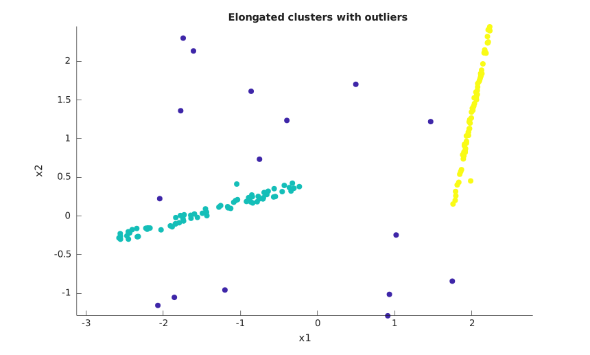
Plot clusters with different shapes and sizes.
f = figure();
rng(12);
n1 = 90;
n2 = 55;
n3 = 70;
theta = 2 * pi * rand(n1, 1);
r = 0.35 * sqrt(rand(n1, 1));
X1 = [r .* cos(theta) - 1.6, r .* sin(theta) + 1.0];
X2 = [0.9 * rand(n2, 1) + 1.2, 0.25 * rand(n2, 1) - 1.1];
X3 = [0.35 * (rand(n3, 1) - 0.5) + 0.5, 1.2 * (rand(n3, 1) - 0.5) + 1.6];
X = [X1; X2; X3];
idx = dbscan(X, 0.28, 5);
c = idx;
c(c < 0) = 0;
scatter(X(:, 1), X(:, 2), 36, c, 'filled');
axis equal;
title('Clusters with different shapes and sizes');
xlabel('x1');
ylabel('x2');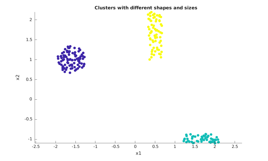
Plot two sinusoidal bands.
f = figure();
rng(13);
n = 140;
t = linspace(-2.5, 2.5, n)';
X1 = [t, sin(1.3 * t)] + 0.08 * (rand(n, 2) - 0.5);
X2 = [t, sin(1.3 * t) - 1.1] + 0.08 * (rand(n, 2) - 0.5);
X = [X1; X2];
idx = dbscan(X, 0.18, 5);
c = idx;
c(c < 0) = 0;
scatter(X(:, 1), X(:, 2), 36, c, 'filled');
axis equal;
title('Sinusoidal bands');
xlabel('x1');
ylabel('x2');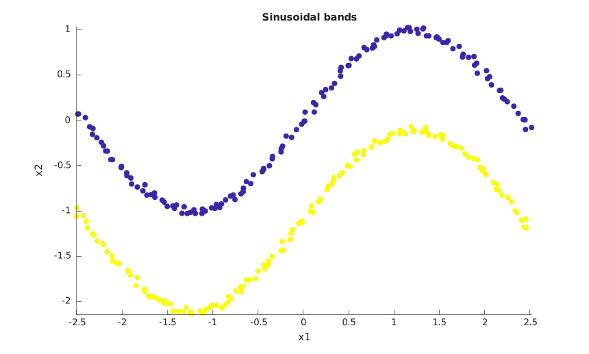
Plot separated arc-shaped clusters.
f = figure();
rng(14);
t1 = linspace(0.2 * pi, 1.55 * pi, 150)';
t2 = linspace(1.85 * pi, 3.15 * pi, 130)';
r1 = 1 + 0.05 * (rand(150, 1) - 0.5);
r2 = 1 + 0.05 * (rand(130, 1) - 0.5);
X1 = [r1 .* cos(t1), r1 .* sin(t1)] + [-1.2, 0.2];
X2 = [1.1 * r2 .* cos(t2), 0.65 * r2 .* sin(t2)] + [1.4, -0.3];
X3 = [4 * rand(20, 1) - 2, 2.6 * rand(20, 1) - 1.3];
X = [X1; X2; X3];
idx = dbscan(X, 0.18, 5);
c = idx;
c(c < 0) = 0;
scatter(X(:, 1), X(:, 2), 36, c, 'filled');
axis equal;
title('Separated arc-shaped clusters');
xlabel('x1');
ylabel('x2');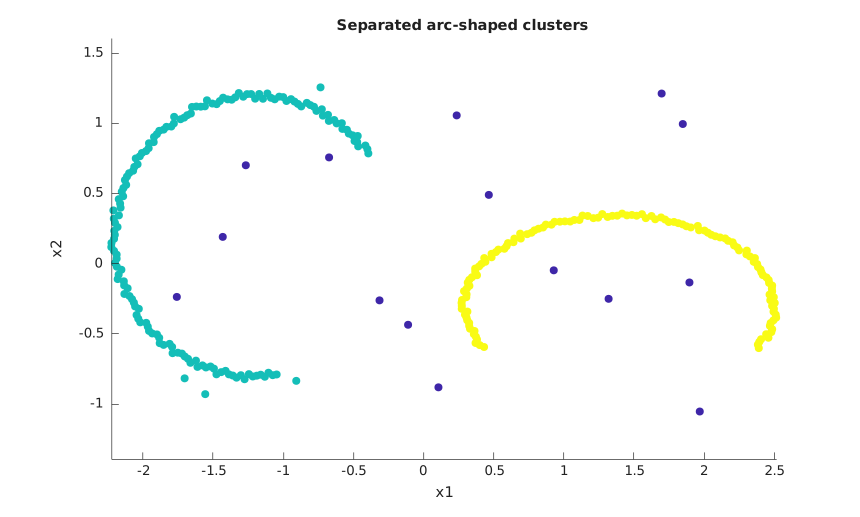
Plot a wavy ribbon and a dense island.
f = figure();
rng(15);
n = 220;
t = linspace(0, 4 * pi, n)';
X1 = [t / (2 * pi) - 1, 0.5 * sin(t)] + 0.07 * (rand(n, 2) - 0.5);
X2 = 0.18 * (rand(80, 2) - 0.5) + [0.8, 1.0];
X3 = [2.8 * rand(20, 1) - 1.4, 2.6 * rand(20, 1) - 1.1];
X = [X1; X2; X3];
idx = dbscan(X, 0.14, 5);
c = idx;
c(c < 0) = 0;
scatter(X(:, 1), X(:, 2), 36, c, 'filled');
axis equal;
title('Wavy ribbon and dense island');
xlabel('x1');
ylabel('x2');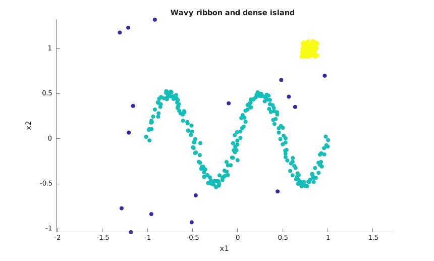
Plot right-angled clusters with the city block distance.
f = figure();
rng(16);
n = 70;
t = linspace(0, 1, n)';
X1 = [[t, zeros(n, 1)]; [ones(n, 1), t]] + 0.04 * (rand(2 * n, 2) - 0.5) - [1.7, 0.4];
X2 = [[-t, zeros(n, 1)]; [-ones(n, 1), t]] + 0.04 * (rand(2 * n, 2) - 0.5) + [1.7, -0.4];
X = [X1; X2];
idx = dbscan(X, 0.16, 4, 'Distance', 'cityblock');
c = idx;
c(c < 0) = 0;
scatter(X(:, 1), X(:, 2), 36, c, 'filled');
axis equal;
title('Right-angled clusters with city block distance');
xlabel('x1');
ylabel('x2');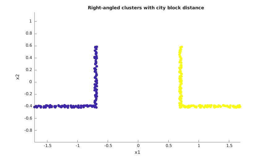
Cluster two rings with the default distance.
N = 90;
theta = linspace(0, 2 * pi, N)';
X = [[0.5 * cos(theta), 0.5 * sin(theta)]; [5 * cos(theta), 5 * sin(theta)]];
idx = dbscan(X, 1, 5)
Handle an empty data matrix.
idx = dbscan(zeros(0, 2), 1, 2)